Page contents
What is the Colebrook-White equation?
The Colebrook-White equation gives the friction factor λ (lambda, also written f) of a pipe in turbulent flow, from the Reynolds number Re and the relative roughness ε/D. It is implicit: λ appears on both sides of the equation, so it is solved by iteration or read from the Moody diagram. It covers every turbulent flow, from smooth to rough pipes, and λ is then used in the Darcy-Weisbach formula to calculate the head loss.
Colebrook-White equation
The friction factor λ then gives the major head loss through the Darcy-Weisbach formula:
- λ: Darcy friction factor, dimensionless (0.01 to 0.08 in practice)
- Re: Reynolds number = V D / ν, dimensionless
- ε: absolute roughness of the wall, in metres (new steel: 0.05 mm)
- D: inside diameter of the pipe, in metres; ε/D is the relative roughness
- L: pipe length, in metres; V: mean velocity, in m/s
- ΔH: head loss in metres of fluid; ΔP: pressure drop in pascals (ΔP = ρ g ΔH)
Haaland's explicit approximation, accurate to about 2 %, is convenient for hand calculations:
Which formula for which flow regime
| Reynolds number | Regime | Friction factor λ |
|---|---|---|
| Re < 2,000 | Laminar | λ = 64 / Re (Poiseuille), independent of roughness |
| 2,000 to 4,000 | Transitional | Unstable: calculate both regimes and keep the worst case |
| 4,000 to 105, smooth wall | Smooth turbulent | λ = 0.316 / Re0.25 (Blasius) or Colebrook |
| > 4,000, any roughness | Turbulent | Colebrook-White (or Haaland), valid in every case |
| Very high Re, rough wall | Fully rough | λ depends on ε/D only: 1/√λ = −2 log10(ε / 3.7 D) |
Detailed explanations and calculation in Mecaflux
The Colebrook-White formula is used to evaluate the coefficient of friction losses in the pipes (Major head loss and linear losses), for all values of the Reynolds number (flow regime)- l is the major head loss coefficient,
- Re is the number of Reynolds
- e = roughness (average size of the roughness of the wall)
- D the pipe diameter
Mecaflux uses this equation for Re > 105
Colebrook charts giving the major losses coefficient (left ordinate) as a function of Reynolds number (x-axis) and the relative roughness (right ordinate) 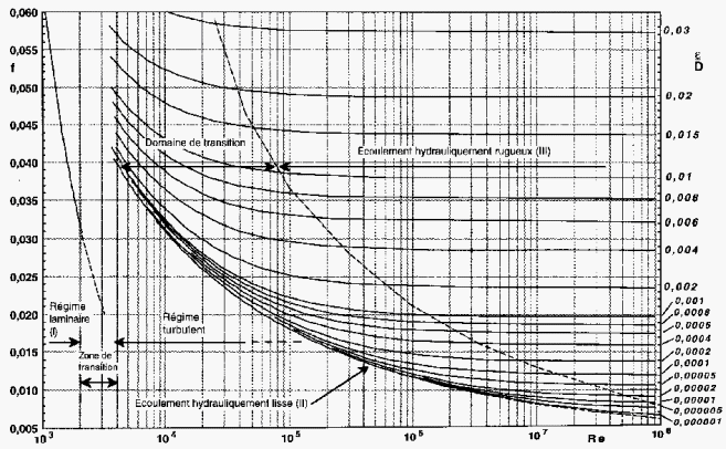
Frequently asked questions
Why is the Colebrook equation implicit and how is it solved?
λ appears on both sides of the equality. Start from an initial value (Haaland's result, or 0.02), compute the right-hand side, deduce a new λ and repeat: three or four iterations are enough. The Mecaflux software does this iteration automatically.
What is the difference between the Colebrook equation and the Moody diagram?
The Moody diagram is the graphical form of the Colebrook-White equation: it plots λ against the Reynolds number for a family of relative roughness curves ε/D. Reading the diagram is the same as solving the equation.
Which roughness should be used in the Colebrook equation?
The absolute roughness ε of the wall, in metres, in the same unit as the diameter: about 0.05 mm for new steel, 0.002 to 0.01 mm for PVC or copper, 1 to 3 mm for corroded cast iron or rough concrete. See the roughness table.
How do I calculate the friction factor of my own pipe?
The major head loss tool of Mecaflux Standard solves the Colebrook equation from the fluid, the flow rate, the diameter and the roughness picked from its table of materials, then gives λ, the pressure drop and the head loss in metres of each run; the inventory then adds up all the runs of the network. For an existing network to diagnose or an extension to size, Mecaflux carries out the study of your project, or offers training on the software applied to your own pipes.